Fetch dataset annotations
This notebook illustrates how to access all the information about a dataset that is visible on the METASPACE platform.
This requires us to:
Connect to the sm server
Select a dataset
Access from the dataset:
Annotations (and their potential metabolites)
Ion images
Optical image
[11]:
import pandas as pd
import matplotlib.pyplot as plt
import numpy as np
Connect to the sm server
The main metaspace2020.eu is configured by default.
[12]:
from metaspace import SMInstance
sm = SMInstance()
[12]:
SMInstance(https://metaspace2020.eu/graphql)
Enter your API Key (only required for private datasets)
To access private datasets on METASPACE, generate an API key from your account page and enter it when prompted below. This step can be skipped for accessing public datasets.
[ ]:
# This will prompt you to enter your API key if needed and it will save it to a config file.
# Note that API keys should be kept secret like passwords.
sm.save_login()
Choose a dataset to visualise
First, we need to select a dataset to visualise. I’ve chosen one of the mouse brain sections from the publication.
Whilst the API does support access by dataset name, it’s most reliable to query using the dataset id. A quick hack to grab this through the web app is to filter the dataset then check the url:

The id for the selected dataset(s) can be copied from here e.g.
http.://metaspace2020.eu/#/annotations?ds=2016-09-22_11h16m17s&sort=-msm
[13]:
dsid = "2016-09-22_11h16m17s"
ds = sm.dataset(id=dsid)
ds
[13]:
SMDataset(Brain01_Bregma-1-46_centroid | ID: 2016-09-22_11h16m17s)
Get a list of the molecular databases used for the dataset annotation.
[14]:
ds.database_details
[14]:
[{'id': 4,
  'name': 'SwissLipids',
  'version': '2016',
  'isPublic': True,
  'archived': True},
 {'id': 22,
  'name': 'HMDB',
  'version': 'v4',
  'isPublic': True,
  'archived': False}]
[20]:
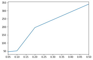
# All results
results = ds.results(database=("HMDB", "v4"))
results.fdr.value_counts().sort_index().cumsum().plot()
plt.show()
# Annotations at 10% FDR
fdr = 0.1
annotations = results[results.fdr <= fdr][['msm']]
annotations.head()
[20]:
| msm | ||
|---|---|---|
| formula | adduct | |
| C40H80NO8P | +K | 0.991456 |
| C43H76NO7P | +Na | 0.987877 |
| C42H84NO8P | +K | 0.987600 |
| C37H71O8P | +K | 0.987128 |
| C44H86NO8P | +K | 0.976368 |
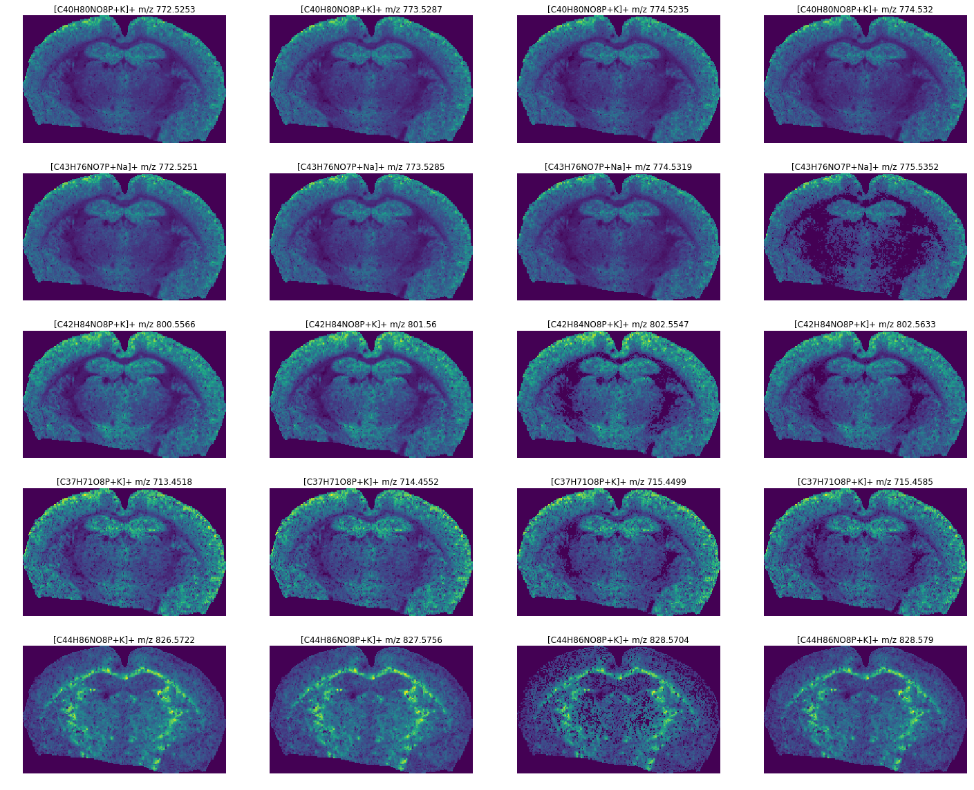
[5]:
limit = 5 # number of annotations to get
plt.figure(figsize=(20, 16))
for ii in range(limit):
    row = results.iloc[ii]
    (sf, adduct) = row.name
    images = ds.isotope_images(sf, adduct)
    for j, im in enumerate(images):
        ax = plt.subplot(limit, 4, ii * 4 + j + 1)
        ax.axis('off')
        plt.title("[{}{}]+ m/z {}".format(sf, adduct, images.peak(index=j)))
        plt.imshow(images[j], cmap='viridis')
plt.tight_layout()
plt.show()
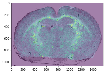
Overlay an ion image on the optical
[6]:
oi = ds.optical_images()
plt.figure()
plt.imshow(oi[0])
plt.imshow(
    np.asarray(
        oi.ion_image_to_optical(images[j])
    ).sum(axis=2),
    cmap='viridis', alpha=0.5)
plt.show()